 One
of the simplest uses of variables is to set up positions from which a set
of milling operations can be performed. In this capacity these variables
work somewhat like the coordinate systems that are common to many g code
implementations.
Introduction
Types of Variables
Units of Variables
Changing Variable Values
Writing blocks using variables
Sample Variable Programs
Example 1 - Drilling a pattern from a variable location
Example 2 - Incremented drilling
Example 3 - An outside milled four cornered object
Example 4 - Milling an inside circle
Example 5 - Iterated Run
Credits
RS274NGC makes provision for the inclusion of variables in the numeric part of program words. Variables can be named with any number up to 5399. You can access the value of a variable in a gcode program by placing a pound (#) sign before the number/name of the variable that you want to reference. Often in the EMC literature the terms variables and parameters are used to refer to the same thing.
For those who learned part programming on older machine tool controls, the inclusion of variables makes for some strange looking program blocks. But variables can be very useful programming tools. This unit develops the concepts of variables as a gcode programming tool and applies them to five common milling tasks.
Before we begin, you need to understand that the NGC development defined
a lot of variables and how they should be used in machine control. But
the EMC and its interpreter only takes advantage of a few of these variables
and those only for its built in coordinate system. You can see which ones,
all in the 5000 + range if you view the emc.var or generic.var files shipped
with EMC. A typical variable file is listed in table 1. We will add and
use several variables that do not have predefined functions in the EMC.
| Format is:
<variable> <value> <variable> runs from 1 to 5399 inclusive, <value> is a number. Units for <value> are INCHES, the default units for RS-274-NGC. Lines not of that form, or blank lines, are considered comments. Don't enter a line beginning with two numbers unless you mean it. You can put whatever you want in here as user variables, but some are reserved. See the RS-274-NGC manual for the reserved variables. This file is loaded into the interpreter at the beginning, and dumped from the controller at the end. Only variables you put explicitly in here will be dumped out from the interpreter.
*columns are used here for display purpose only. They are not supported in the .var file itself. |
There are two ways to define variables for use in part programs. The most obvious is an explicit reference to the variable in the currently used variable file. Each time the EMC starts up it loads a variable file. The default variable file is emc.var but this can be changed in the .ini file. For convenience, this paper uses emc.var as if it were the currently loaded file.
When the following line is placed in emc.var, it explicitly defines a variable.
1000 55The number 1000 is the name of the variable, and once you have defined it and read it into the interpreter, you can use that name in your g-code program if you place a pound sign in front of it. With the line above, we also assigned variable #1000 the value of 55 by placing that number on the same line after the variable name. Any time that you name a variable and assign a value to it in emc.var you have explicitely defined that variable.
Implicit reference to a variable is done when a name is used within a program but no reference is made to that variable in the variable file. The following line of code in a part program will initialize a variable named 1000 and assign it a value of 55.
#1000 = 55Implicit variables initialize to zero value if no assignment is made before a variable is first used. Implicit variables disappear when the EMC interpreter is shut down but will hold a current value as long as the EMC is running.
Explicit variables act just like implicit variables while the EMC is running but reloading the variable file will reset explicit variables to the value that they are assigned in the variable file. When EMC is shut down normally, the current values of all explicit variables are written into emc.var. Since explicit variables can change value from one run of EMC to the next, they may not contain the values that you expect when you restart your machine.
The EMC doesn't care very much what we name variables or what we use them for. For explicitly defined variables, the EMC cares only that they are two numbers in a row on a line by themselves in the emc.var file. For implicitly defined variables, the EMC cares not a whit. The only complaints that you might get from the EMC is if a reference to a variable makes a reference to an unknown word, or is out of range for a distance, or concerns tool compensation. While you are writing or using variables you will want to refer to and probably stay away from those variables listed in emc.ini that are used to set up the coordinate systems.
Units of VariablesNo units are implied by the value assigned to a variable. Variables simply contain numbers. As an example, if variable #1000 as we have defined it above were referenced in a part program after a (g) as we have done in the following line, it would refer to a coordinate system. In this case g55.
G#1000If it were referenced after an (x, y, or z) it would refer to a positive distance on the named axis. That distance would depend on whether you had defined distance in inches or millimeters or some other unit.
X#1000If #1000 were referenced after a (b) for a rotary axis it would refer to a positive rotation of 55 degrees. And if it were referenced after a (t) it would refer to a tool slot.
T#1000 M6One consequence of the valuelesness of variables is that they will change meaning when you change from inches to millimeters in a program. Changing Variable Values
The variable assignment operator allows you to change the value of a variable while a gcode program is running. Any reference to a variable name followed by an equals sign and a number or an expression in brackets [] will assign that number to the named variable.
#1002 = [#1000 + #1001]In the case of the previous line, #1002 takes on the value of the sum of two other variables. Variables can be assigned any values that can be computed within a program.
One interesting case of assignment comes from the fact that you can assign a variable it's own value so incrementing is permitted by the interpreter.
#1000 = [#1000 + 1]If you increment or change a variable while a program is running it will hold its new value for the next run of the same program. It will continue to hold the last value when you start a different program. Writing blocks using variables
Right about now, the conventional program code writer will realize that it is a bit easier to just write the real numbered code than it is to write the variable code. It is also easier to read and make sense of real numbered code as the following two lines illustrate.
Hard code T55 M6 G43 H55 G55 X55 A55And real numbered code will take less time to write if you want to use that code or those numeric values only one time. The real value of code written with variables becomes obvious if you want to re use code for different sized parts, past in the same code several times, or when using different setups and tools.
Variable code T#1000 M6 G43 H#1000 G#1000 X#1000 A#1000
Variables can also be of value where a location is repeated many times during a program. Rather than typing (x21.1345) in a dozen locations in a program you can assign that value to a variable at the top of your program and reference it wherever you need to within. Then if a program wide change needs to be made to that value it can be done once and all references will shift to the new value.
Under any of these conditions variable programming becomes much more efficient than repeating or editing all those lines of code with the correct values.
In this section we develop five examples of the use of variables in program code. These examples are not intended to be complete in themselves. Nor are they intended to be particularly useful or efficient. They are intended only to illustrate certain uses of variables in gcode.
You should also remember that these code samples were all written for
my machine. It does not lay out the axis the way that they are on graph
paper. X moves plus toward the left and y moves minus toward you when you
face the mill. For all of the illustrations below the operator would be
standing below the figure and looking into it.
Example 1 - Drilling a pattern from a variable location
 One
of the simplest uses of variables is to set up positions from which a set
of milling operations can be performed. In this capacity these variables
work somewhat like the coordinate systems that are common to many g code
implementations.
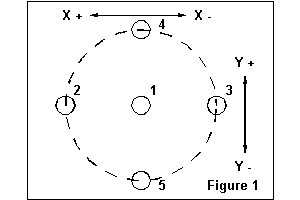
This program assumes that the drill bit is already loaded and that the machine is home. The pattern is five holes. One in the center and four on a 1 inch radius around that center hole. Opposite holes in the pattern are aligned with the axes in what could be called a diamond. (see figure 1)
We will begin by assigning values to two variables. We can then use these variables as the center of the hole pattern and increment the drilling operation with respect to that center location.
| N10 #1000 = 4.5120 (x distance for center of set of 4
holes)
N12 #1001 = 2.6873 (y distance for center of set of holes) N14 g0 x#1000 y#1001 z1 (move to center location) N16 g1 f4 z2 (drill center hole) N18 g0 z0 N20 x[#1000 + 1.0] (move to first diamond hole) N22 z1 N24 g1 f4 z2 (drill first diamond corner hole) N26 g0 z0 N28 x[#1000 - 1.0] (move to second diamond hole) N30 z1 N32 g1 f4 z2 (drill second diamond corner hole) N34 g0 z0 N36 x#1000 y[#1001 + 1.0] (move to third diamond hole) N38 z1 N40 g1 f4 z2 (drill third diamond corner hole) N42 g0 z0 N44 y[#1001 - 1.0] (move to fourth diamond hole) N46 z1 N48 g1 f4 z2 (drill fourth diamond corner hole) N50 g0 z0 N52 g53 x0 y0 z0 N54 m2 |
This set of code blocks could have been written using the real values for the locations, however the use of just two variables allows the entire pattern to be shifted rather easily during production to keep the hole locations within the tolerances specified on the print. Writing this kind of code using variables also allows for wide variation in the setup of the machine for milling.
In this example the pattern is a fixed shape and size - perhaps a pipe flange or a bearing mount for a sliding rod. The two variables allow the operator to quickly shift the pattern to the exact coordinates where it should be placed. In the example the editing would have to be done to the program code on lines N10 and N12 because the variables are implicit. Explicit variables would allow the operator to change the values in the emc.var file and reload it.
Code like that developed in this example can easily be copied and pasted several times into the same program to reproduce the same pattern at several locations. The only additional code that must be added is a line that changes the variables for each location. This could be as simple as #1000 = (number) before each pasted chunk, or it could be an increment from the first location. Example two shows how to increment.
Example 2 - Incremented drillingThe lines of code in table 3 illustrate the technique of incrementing variables along with using those variables during the running of a program. Again lines N10 and N12 assign initial values to the variables that will be used. Line N14 moves the machine to the location of the hole to be drilled while N16 and N18 perform the operation. Line N20 increments both variables. In the illustrated code #1000 is increased by 2 and #1001 is increased by 1. Taken together, lines N14 through 18 are a loop (although this version of RS274NGC does not implement looping) and the code is just copied and pasted into the program for the number of times the operation is to be repeated.
| N10 #1000 = 0 (x distance for first hole)
N12 #1001 = 0 (y distance for first holes) N14 G55 g0 x#1000 y#1001 z1 (move to first hole) N16 g1 f4 z2 (drill) N18 g0 z0 N20 #1000 = [#1000 + 2] #1001 = [1001 + 1] N14 G55 g0 x#1000 y#1001 z1 (move to second hole) N16 g1 f4 z2 (drill) N18 g0 z0 N20 #1000 = [#1000 + 2] #1001 = [1001 + 1] N14 G55 g0 x#1000 y#1001 z1 (move to third hole) N16 g1 f4 z2 (drill) N18 g0 z0 N20 #1000 = [#1000 + 2] #1001 = [1001 + 1] N14 G55 g0 x#1000 y#1001 z1 (move to fourth hole) N16 g1 f4 z2 (drill) N18 g0 z0 N52 g53 x0 y0 z0 N54 m2 |
Since the EMC interpreter doesn't care what the lines are numbered, the above code will run as is. It would look somewhat better if it were renumbered. Again only the variable values need to be changed to move the location of the set of holes. In this case, the code will produce a diagonal set of four holes. Each hole is two inches in x and one inch in y away from the previous hole.
A cautionary note must be included here. Once the machine tool is into the program, there is no good way to know where it is except to observe the machine itself. Stopping and then restarting from anywhere but the top line is an invitation to disaster because the values of the variables have been changed by the program itself.
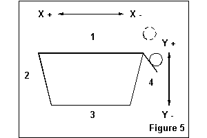
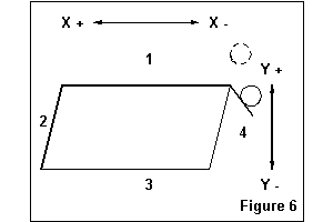
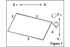
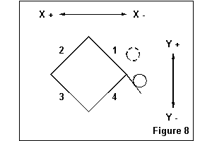
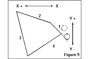
Example 3 - An outside milled four cornered object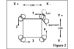 This
example is more complicated than what you have seen so far. Our task is
to mill a four cornered object that has all outside corners using tool
diameter compensation. This object could be a square, a rectangle, a parallelogram,
a trapezoid, or an object where none of the angles and sides are the same.
We need to tell the machine all of the following information.
| N0130 g53 g0 x0 y0 z0 (send the machine to machine home)
N0140 g17 t1 m6 m0 (load tool 1) N0150 g40 h1 g55 x0 y0 z0 (pick up tool length and move to coordinate home) N0160 x-1 y-0.5 (45 degree approach point with 0.5 tool radius offset) N0170 z-2.5 (milling depth) N0180 g1 f10 g41 x0 y0 m8 (approach first corner with coolant) N0190 x2 (mill first side) N0200 y-2 (mill second side) N0210 x0 (mill third side) N0220 y0 (mill fourth side) N0230 g49 y0.25 m9 (turn off comp and coolant and clear part) N0240 g0 z0 (retract z) N0250 g53 x0 y0 z0 (move back to machine home) N0260 M2 (program end) |
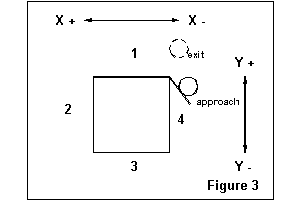
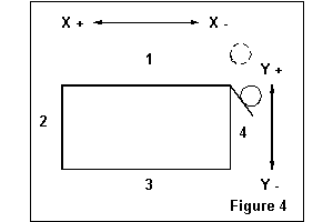
The size and shape of the part can be changed and depend upon the actual numbers entered in lines numbered 190 to 220. Suppose we wanted to cut a trapezoid with the small side one inch less that the long side. This could easily be made trapezoidal by changing those lines as table 5 lists. A set of these sample shapes is shown in table 8.
| N0190 x2 (mill first side)
N0200 x1.5 y-2 (mill second side) N0210 x0.5 (mill third side) N0220 x0 y0 (mill fourth side) |
Now the narrow side is one inch smaller than its longer parallel side and the other two are angled in by a half inch. Notice that very few changes needed to be made in the code in order to create the second part. We added both coordinates to the corner definitions and changed the actual numbers. These distance kinds of g-code numbers can be stored as variables. By changing the actual values of these variables we can create many different sizes and shapes using the same set of part program code.
First we need to define a set of variables and what we will use them for.
| 1000 Tool Number
1001 Tool Diameter 1002 Coordinate Reference 1003 Finished depth of cutter 1004 First corner x location 1005 First corner y location 1006 Second corner x location 1007 Second corner y location 1008 Third corner x location 1009 Third corner y location 1010 Fourth corner x location 1011 Fourth corner y location |
One small problem that comes up with variable programming is that often you must include the tool diameter both in the tool file and as a variable when it will be used to compute an approach point.
Now all that we have to do is plug in these variable names in place of the hard numbers in the above code. For this more general case, we will include x and y coordinates for each corner. By doing this we can rotate the shape and make non parallel sides. We will also need to set up a computation for the approach in line 40 and the exit in line 110.
The variables and what they do are included in code as comment blocks. This way if the part program and the variable file become separated I can recreate the variable file easily. Including the variables as comments also helps when reading the program and debugging a setup.
| n10 (1000 Tool Number)
n20 (1001 Tool Diameter) n30 (1002 Coodinate Reference) n40 (1003 Finished Depth of cut) n50 (1004 First corner x location) n60 (1005 First corner y location) n70 (1006 Second corner x location) n80 (1007 Second corner y location) n90 (1008 Third corner x location) n100 (1009 Third corner y location) n110 (1010 Fourth corner x location) n120 (1011 Fourth corner y location) n130 g0 g53 x0 y0 z0 (machine home) n140 g17 t#1000 m6 m0 (load tool) n150 g43 h#1000 G#1002 x0 y0 z0 (move to offsets) n160 x[-1*#1001] y[-1*[#1001/2]] (45 degree approach) n170 z[-1*#1003] (tool to depth) n180 g1 f10 g41 d#1000 x#1004 y#1005 m8 (comp, cool, and approach corner) n190 x#1006 y#1007 (mill first side) n200 x#1008 y#1009 (mill second side) n210 x#1010 y#1011 (mill third side) n220 x#1004 y#1005 (mill fourth side) n230 g40 y[#1001/4] m9 (clear part) n240 g49 t0 m6 g0 z0 n250 g53 x0 y0 z0 n260 m2 |
There are some limits on how far you can rotate this part using the four corners. A useful rule is that the line between the first corner and the second should not be more than 45 degrees off of the x axis of the machine or the cutter comp may not work correctly. If the line between the last corner and the first is steeper than a 45 you will get a tool gouge that will not be reported by the EMC.
|
 |
|||||||||||||||
|
 |
|||||||||||||||
|
 |
|||||||||||||||
|
 |
|||||||||||||||
|
 |
|||||||||||||||
|
 |
|||||||||||||||
|
 |
As mentioned earlier, this code and the shapes that can be cut with it is not very easy to read. But you should read through it and substitute the variable description wherever you find a pound sign. When you have done this a few times any program file that uses variables will become easier to understand.
Example 4 - Milling an inside circleInside milling with cutter compensation requires a little more complexity on the approach and setup of the cutter compensation but the use of variables works much the same way that it did in the four sided example above.
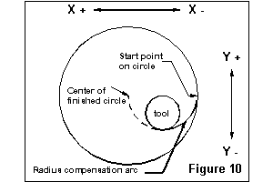 For
this example we want to drill an initial hole inside the circle and then
change to the end mill and return to the hole and start the approach there.
The first step is to list the steps that we need to take to complete this
task.
For the initial test of this program, the relevant portion of the variable file looked like those lines in table 9.
| Coordinate system to use is variable 1100.
1100 56 Drill pocket number in variable 1101 below.
Mill pocket number in variable 1102 below.
Finished Hole Diameter in variable 1103 below.
End Mill Diameter in variable 1104 below.
|
By using variables we are able to easily adjust the size of the hole that will be cut and the size of the cutter. By making the tool slots also variables, the code can be used over and over in the same program with different combinations. Editing sizes is relatively easy for the operator during final setup and run because the variables are explicit. One caution here is that both #1104 and the size of the tool defined in the emc.tbl need to be about the same size.
Example 4 uses one half of the radius of the finished circle as the radius of the tool approach for tool diameter compensation. (see figure 11) The edge of the tool is placed on this arc before the compensation move is begun. For large circles this approach may waste some time getting from the initial location to the start of the circle cut. A change in the approach point arithmetic expression could move the approach point closer to the edge of the circle.
| n010 (Var #1100 is coordinate system number)
n020 (Var #1101 is drill tool slot) n030 (Var #1102 is mill tool slot) n040 (Var #1103 is hole diameter) n050 (Var #1104 is tool diameter) n060 g#1100 g0 x0 y0 z0 (machine home from previous work) n070 (place your tool load routine about here) n080 g55 t#1000 m6 g43 h#1000 (pick up drill and offsets for this hole) n090 x[#1002/4] y[-1*[[#1002/4]-[#1003/2]]] z0 (move to initial position) n100 G1 f5 z-1 (drill starting hole) n110 f25 z0 (retract quill) n120 g53 g0 x0 y0 z0 (go back to tool change position) n130 (place your tool load routine about here) n140 t#1001 m6 g43 h#1001 (pick up mill) n150 x[#1002/4] y[-1*[[#1002/4]-[#1003/2]]] z0 (mill to initial position) n160 G1 f5 z-1 (mill starting hole) n170 g17 g41 d2 G3 f3 x[#1002/2] y0 r[#1002/4] (offset arc to start) n180 x[-1*[#1002/2]] r[#1002/2] (cut the first half circle) n190 x[#1002/2] r[#1002/2] (cut the second half circle) n200 g40 t0 m6 g43 h0 g0 z0 (drop offsets and retract quill) n210 g53 g0 x0 y0 z0 (go home) n220 m2 |
One limitation of the code in table 10 is that tool diameter can't be larger than the radius (d/2) of the finished hole or the EMC will generate a cutting compensation error message.
Example 5 - Iterated RunAs we have already seen in example 2, the EMC's interpreter allows for the setting of variables during program code execution. That example reset the loop variable at the start of each program run. But the value of a variable persists throughout the life of an EMC run so that it's incremented value can be accessed by pressing the <run> button to start the next loop.
Variable #1000 is a explicit variable. It is also the loop variable. By making #1000 explicit the machine operator can reset the loop to zero by reloading the parameter file from the TclTk parameter edit window when all of the loops through the program have been completed. This code shows a simple drilling operation that uses successive coordinate systems for each run.
This line is placed in the variable file.
1000 1001The code in table 11 shows a simple drilling operation that uses successive coordinate systems each time the run button is pressed. It is line number n150 that does the work of incrementing explicit loop variable #1000. The work done by the machine could be expanded with the addition of lines of code before line 150 to as large a program as needed at each coordinate position.
| n10 (sample loop program with <run> press for each
interation)
n20 #1001 = 54 (variables to reference coordinate systems) n30 #1002 = 55 n40 #1003 = 56 n50 #1004 = 57 n60 #1005 = 58 n70 #1006 = 59 n80 #1007 = 59.1 n90 #1008 = 59.2 n100 #1009 = 59.3 n110 g0 x0 y0 z0 (move to known location) n120 g#[#1000 + 1001] x0 y0 (pick up new coordinates) n130 g1 f5 z1 (drill) n140 g0 z0 n150 #1000 = [#1000 + 1] Increment the loop variable) n160 m2 |
This kind of program might be used with a setup that had a number of vices on the milling table with the same part in each. The same thing could be achieved using a single program with incrementing between each and an option stop (m0). Such a program would be much longer and would require <restart> rather than <run>.
As the EMC interpreter exists now, there is no good way to know which coordinate system will be used next without looking at the machine or remembering the offsets as loaded into each coordinate system. This code will also cause an error message if you attempt to run it after the nineth time. Since the loop variable is explicit, it can be reset at any time before the EMC is shut down by reloading the variable file.
This page is a part of the EMC Handbook and is covered by its GPLD
copyright. It is maintained by Ray
Henry. Comments, criticism, flames, additions, subtractions, and editing
are welcomed.